GSL Paper Explainer: Using simulations to demonstrate the importance of considering variation within sexes in genetics
Human evolutionary history is defined by movement and mixture at many scales: between communities, continents, and even across species. While the causes of the events that bring groups into contact vary wildly, geneticists have built quantitative frameworks for inferring some of the demographic properties of these events – such as the sex ratio of migrating individuals – without needing to know the exact mechanisms under which they occurred. This assumption of interchangeability is a common modeling strategy which treats sex as what we term a “shorthand” for the constellation of unknown factors that generate an observed sex ratio in a demographic event.
In a new paper in the American Journal of Human Biology by Mia Miyagi, Sarah Richardson, and Emilia Huerta-Sánchez from the Center for Computational Molecular Biology at Brown, we explore the effect of variation within a sex on these inference methods and use simulations to demonstrate that this variability can affect common variables used to quantify the sex ratio of migration events. Our results highlight that modeling individuals of the ‘same’ sex as interchangeable can have quantitative consequences and represent an application of sex contextualist principles to an open area of research in human biology.
In this explainer, we’ll walk through:
(1) How scientists use X chromosomes to infer the sex ratio, or sex bias, of migration events.
(2) How we simulated the impact of variation within sexes on this inference.
(3) Why this serves as an example of the quantitative importance of feminist approaches to sex in evolutionary biology.
Sex-biased migration is usually inferred using X chromosomes
Inference of sex-biased migration starts with an assumed correspondence between an individual’s chromosomes and sex, such that a certain chromosomal conformation (e.g. ‘XY’ or ‘XX’) maps to a specific sex category (e.g. ‘male or ‘female’). With this correlation between sex and chromosomes set, these methods then look for differences in the evolutionary history or ancestry of chromosomes, which are interpreted as reflecting differences between sexes. For example, Neanderthal ancestry is slightly lower on the X chromosome than the autosomes in modern humans, an observation which is often interpreted as suggesting that Neanderthal males were more likely to have children with modern human females than vice versa (Juric et al. 2016).
To understand this, imagine an ancestral population has split into two different populations (Figure 1a), which are usually not in contact. At some point in the past, a migration event moves individuals from Population 1 (orange) into Population 2 (blue), indicated by an arrow. After the migration event, some individuals in Population 2 are descended from individuals from Population 1. Intuitively, the frequency of these individuals tells us something about the number of individuals that migrated in the original event, even after generations pass.
There is an additional wrinkle when thinking about real data, as not every chromosome in an individual has the same ancestry. For example, half of your genome can be traced through each of your parents, and these halves do not have the same genealogy. While this is a complication, it is a helpful one, as it means we can look for meaningful differences in average ancestry throughout the genome. Similarly to the individual level, the ancestry of chromosomes in Population 2 tells us something about the number of that chromosome that migrated (via an individual) in the migration event.
For any chromosome that is present in every individual in the population (e.g. the autosomes, or any chromosome that is not a sex chromosome), we’d expect that their ancestry should look fairly similar to each other. But for the X and Y, the fraction of chromosomes which trace their lineage to Population 1 depends on the number of X’s and Y’s present in the migration event, and therefore this fraction is usually assumed to correlate with ‘sex’. In this way, the average ancestry of the X chromosomes and autosomes can differ. In theory, this difference then tells us something about the separate evolutionary histories of each sex (Figure 1b). For example, if the X chromosomes have more Population 1 ancestry than the autosomes, it is generally inferred that X chromosomes were overrepresented in the migrating individuals, or that there were more XX individuals than XY individuals who migrated.
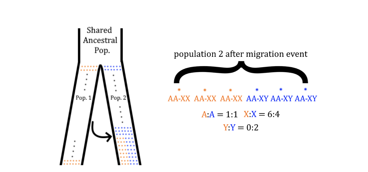
Figure 1: Panel A shows a history where two populations (1 and 2) diverge from each other and exist independently until a migration event moves individuals from Population 1 into Population 2. In Panel B, we look at a single generation in Population 2 after the migration event, with each individual’s chromosomes labeled. While the autosomes’ (‘A’) ancestry matches the population-wide ratio, the X and Y chromosomes do not, as all the migrating individuals are XX.
We found that modeling sex-biased migration without individual variation within a sex underestimates the variance on estimates of sex bias in migration – it can be higher than people think!
The model above allows us to think about a correspondence between chromosome-by-chromosome ancestry to the sex ratio of a migration event. However, the reliability of this mapping depends on whether it holds under various potential deviations from the idealized model. It has been previously shown, for example, that if the migration event is not instantaneous, but instead takes multiple generations, it results in different population ancestry than a single pulse of migration (Goldberg and Rosenberg 2015).
We were interested in a different deviation from the ideal: what if not all individuals within a sex have the same probability to migrate? Using simulations, we tested multiple models where an individual’s migration probability was determined not just by sex, but by either genetic factors or geography. Here, we’ll focus on the geographic model. In these simulations, we selected migrants clumped by proximity, such that individuals closer to each other are more likely to either both migrate or both remain in their original population (Figure 2). In each case, we compared the resulting X chromosome ancestry to a control simulation with a migration event with the exact same number of male and female migrants, but where all migrants were selected completely at random within a sex.
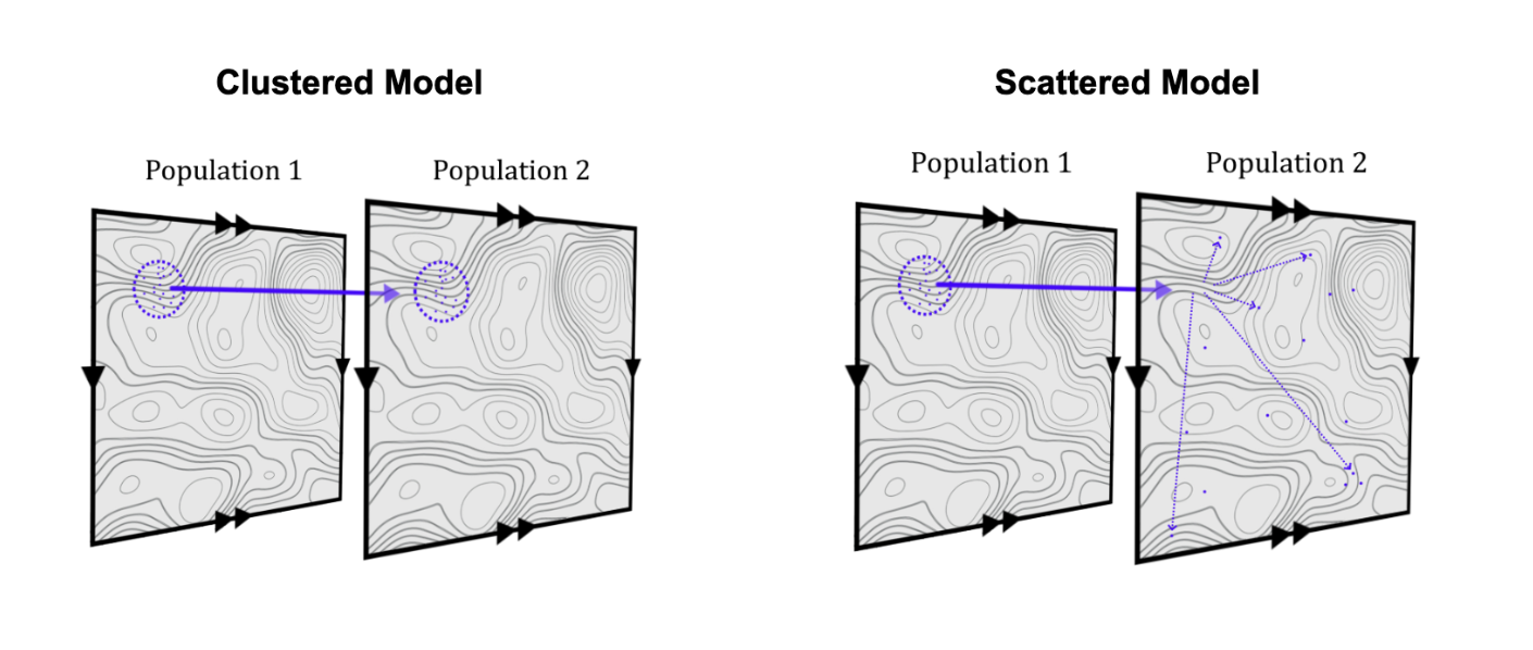
Figure 2: A schematic of our geographic simulation models, where a clump of individuals are selected to migrate from Population 1 into Population 2. To control for potential effects of density, we tested a case where migrants were transplanted from population 1 into 2 with their coordinates preserved (Panel A), and another where migrants were dispersed after joining population 2 (Panel B). Other fun are considerations detailed in the paper text!
If variability within a sex has no bearing on ancestry patterns on the X chromosome after a migration event, then we would expect that the control (where individuals are selected at random) should look identical to the tests where individuals can vary in their migration probability. However, we find that this is not the case in both the genetic and the geographic model (for example, Figure 3). We don’t know for certain what causes this discrepancy, but some of our simulations indicate it may result from these migrant selection processes affecting the average relatedness of the migrating individuals. Fundamentally, this result means that two migration events with equal sex ratios might result in different X-ancestry distributions depending on the process which drives the migration.
This result has implications for how we compare and create narratives about the role sex played in historic migration events. Imagine we know that sex or gender interacts with geography in determining which individuals choose to migrate between populations. This could be due to localized cultural pressures, differences in economic ability to move, or other idiosyncratic factors. If these induce different geographic patterns of movement (such as in Figure 2), our result implies that using X chromosome ancestry alone to describe one event as “more sex-biased” than another may not be as accurate as assumed.
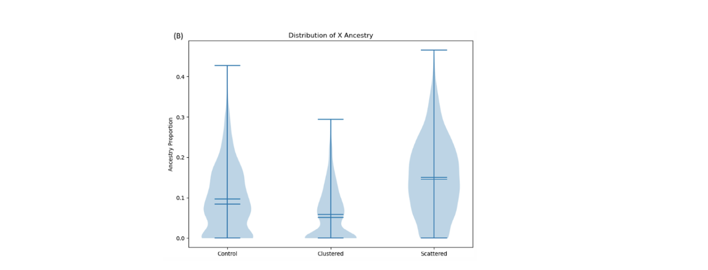
Figure 3: A panel from our results comparing the two geographic models from Figure 2 to the control. Proportion of ‘Population 1’ ancestry on the X chromosome is shown on the Y-axis. We claim these distributions are statistically (and visually) distinct. For quantitative details, please see the paper!
Proof of concept for a sex contextualist framework for reasoning about sex categories in human biology
On a more general level, our paper argues that this is an example of how sex contextualism, a framework which treats sex as context-dependent and plural, can aid in the generation of new scientific questions (Shattuck-Heidorn and Ichikawa 2022). In this case, sex contextualism highlights that the choice of how one models variation within a sex is exactly that – a choice. This motivates us to actively simulate processes which might differentially affect individuals within a sex category. By doing that, we find that (in this context) modeling individuals within a sex as exchangeable has quantitative consequences, and that two migration events which are demographically identical with respect to sex (i.e. equally sex-biased) look different at the genomic level depending on how this bias is generated. In other words, while previous work has largely modeled sex-biased demographic events as disparate as firefly migrations (Catalán et al. 2025) and internal movement of people within the US (Bryc et al. 2015) using some of the same tools, we suggest that describing both of these as simply ‘sex-biased’ flattens important variation in mechanism between them.
Sex contextualism gives us a toolkit for critical engagement with how research around sex and sex differences is conducted and reported. We hope this case shows how this criticality can benefit scientists in the formulation of new research questions and simulation models, a frontier we will continue to explore in our future work.
Read the full article here: Miyagi, M., E. Huerta-Sánchez, and S. S. Richardson. 2025. “ Contextualizing Population Genetic Models of Sex-Biased Migration and Admixture.” American Journal of Human Biology 37, no. 12: e70183. https://doi.org/10.1002/ajhb.70183.
STATEMENT OF INTELLECTUAL LABOR
This blog post was drafted by Mia Miyagi with edits and feedback from Sarah Richardson, as well as comments and input from all members of the GenderSci Lab.
RECOMMENDED CITATION
Miyagi, M. and Richardson, S.S. “GSL Paper Explainer: Using simulations to demonstrate the importance of considering variation within sexes in genetics.” Gendersci Lab Blog. 10 February 2026. https://www.genderscilab.org/blog/gsl-paper-explainer-using-simulations-to-demonstrate-the-importance-of-considering-variation-within-sexes-in-genetics.